Mixed Precision Training

`float32` v/s `float16` v/s `bfloat16`

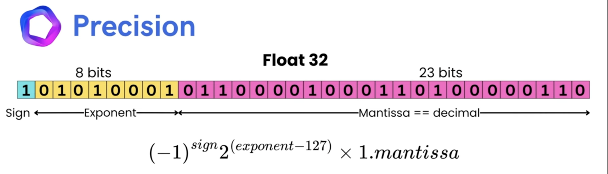
Precision comparision

float32

float32

float16 & bfloat16 & float8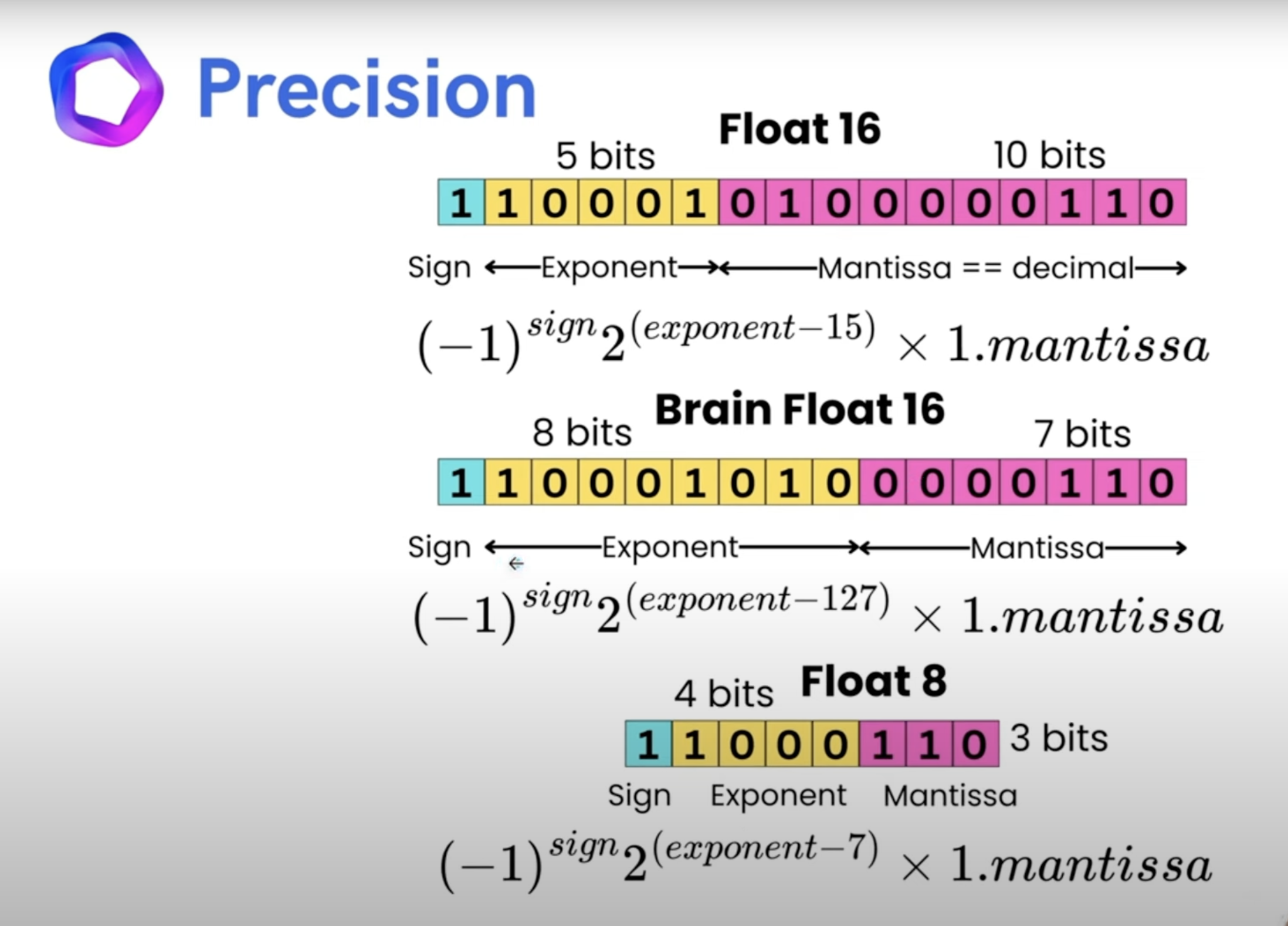

<ul> <li><code>float32</code> & <code>bfloat16</code> have similar range, but <code>float32</code> has higher precision.</li> <li><code>float16</code> has both lower range & precision compared to <code>float32</code>.</li> <li><code>float16</code> has a smaller dynamic range compared to <code>bfloat16</code>, but <code>bfloat16</code> has lower precision.</li> </ul>

Range Comparison

range of different float types

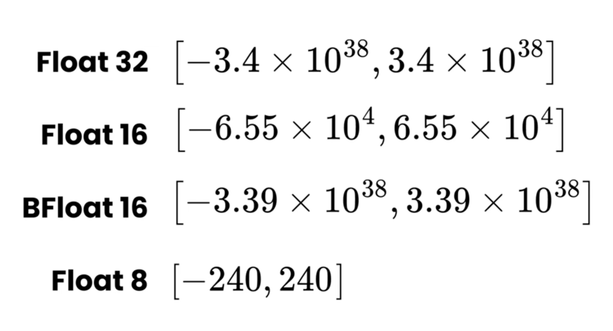
<code>Note</code>: <code>bfloat16</code> & <code>float32</code> have similar ranges, but <code>float32</code> has higher precision.

Converting datatype

f32 to f16

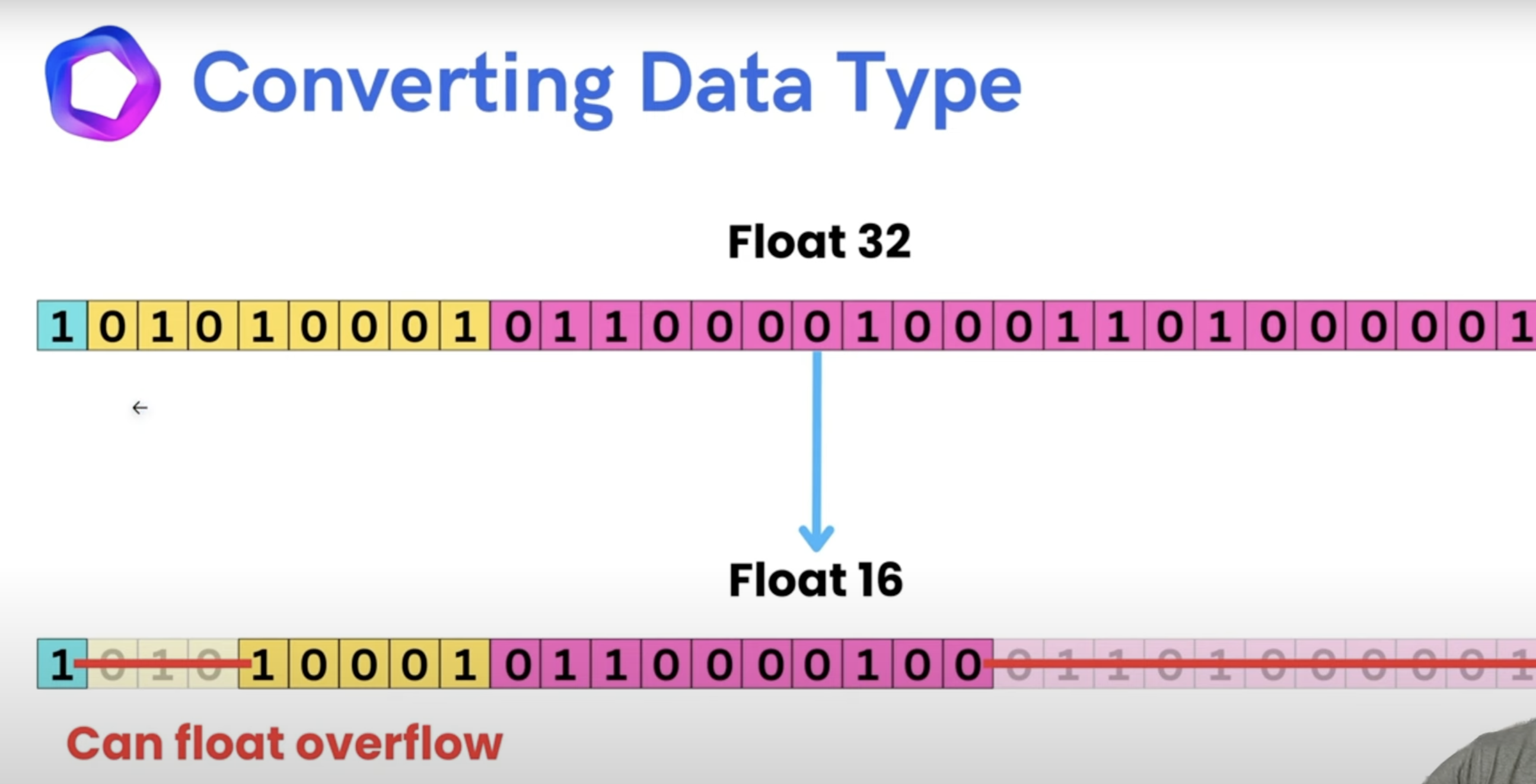
has risk of overflow

f32 to bf16

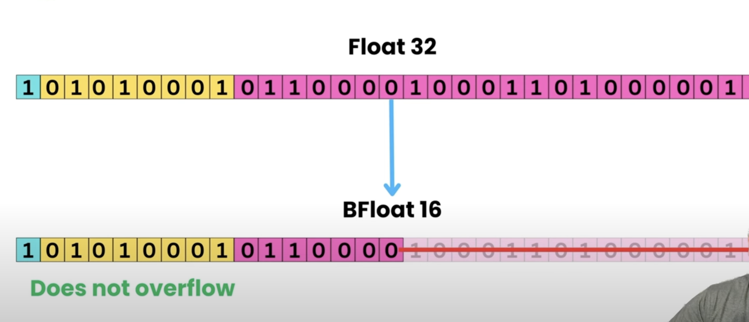
doesn’t overflow

Mixed Precision Training in PyTorch

Mixed precision training is a technique that combines the use of both 16-bit (half precision) and 32-bit (single precision) floating-point representations during training to accelerate training while maintaining model accuracy.

Mixed precision training can provide up to 1.5-2x speedup on modern GPUs with Tensor Cores (V100, A100, RTX series) while reducing memory usage by approximately 50%.

What is Mixed Precision Training?

Mixed precision training uses lower precision (FP16) for most operations while keeping higher precision (FP32) for operations that require it. This approach:

Speeds up training by leveraging specialized hardware (Tensor Cores)
Reduces memory usage by storing activations and gradients in FP16
Maintains training stability by using FP32 for loss scaling and parameter updates
Preserves model accuracy through careful handling of numerical precision

Key Concepts

1. Automatic Mixed Precision (AMP)

PyTorch’s AMP automatically decides which operations should use FP16 vs FP32 based on:

Safe operations: Matrix multiplications, convolutions → FP16
Unsafe operations: Loss functions, softmax, layer norm → FP32

2. Loss Scaling

FP16 has a smaller dynamic range than FP32, which can cause gradient underflow
Loss scaling multiplies the loss by a large factor before backpropagation
Gradients are unscaled before optimizer step to maintain correct magnitudes

3. Gradient Scaling and Unscaling

Scaling: Prevents gradient underflow by amplifying small gradients
Unscaling: Restores original gradient magnitudes before parameter updates
Dynamic scaling: Automatically adjusts scale factor based on gradient overflow detection

Basic Mixed Precision Training

import torch
import torch.nn as nn
import torch.optim as optim
from torch.cuda.amp import autocast, GradScaler

# Model, loss, optimizer
model = nn.Linear(1000, 10).cuda()
criterion = nn.CrossEntropyLoss()
optimizer = optim.Adam(model.parameters(), lr=1e-3)

# Create gradient scaler for mixed precision
scaler = GradScaler()

# Training data
data = torch.randn(64, 1000).cuda()
targets = torch.randint(0, 10, (64,)).cuda()

model.train()
optimizer.zero_grad()

# Forward pass with autocast
with autocast():
    outputs = model(data)
    loss = criterion(outputs, targets)

# Backward pass with scaled loss
scaler.scale(loss).backward()

# Optimizer step with gradient unscaling
scaler.step(optimizer)

# Update scaler for next iteration
scaler.update()

print(f"Loss: {loss.item():.4f}")

Key Components Explained

autocast(): Context manager that automatically casts operations to appropriate precision
GradScaler(): Handles loss scaling, gradient unscaling, and dynamic scale factor updates
scaler.scale(loss): Scales loss before backward pass to prevent gradient underflow
scaler.step(optimizer): Unscales gradients and performs optimizer step if no overflow
scaler.update(): Updates the scale factor for next iteration

What actually happens in `Mixed-Precision` training?

The Mixed Precision Training Workflow

The training process is a loop that repeats for every batch of data. Here is what happens inside a single training loop with mixed precision:

1. The Forward Pass

Action: A temporary float16 copy of the weights is created. The input data is also converted to float16.
Calculation: All the computationally-heavy operations (matrix multiplications) are performed using float16. This is much faster on modern GPUs with special hardware like Tensor Cores.
Memory Impact: The intermediate outputs, called activations, are also stored in float16. Since activations take up a huge amount of memory, this is the main source of the memory savings.

[ Diagram: Forward Pass ]

--------------------->>
 Input Data (float32)

    [ Convert to float16 ]
                 v
                 v
                 +-------------------+
                 | Model (in float16)| <--- [TEMPORARY]
                 |   - Weights       |
                 |   - Biases        |
                 +-------------------+
                 | Activations       | <--- [STORED in float16]
                 | Gradients         |
                 +-------------------+
                 v
         Output (float16)

2. Loss Scaling

Action: The float16 output from the forward pass is used to calculate the loss. This loss is then multiplied by a large number (the “loss scaler”).
Calculation: loss = loss * scaler
Why? The gradients for some layers can be extremely small. If they were in float16, they would be rounded to zero, causing the model to stop learning. By scaling up the loss, all the gradients that are calculated in the next step are also scaled up, so they don’t disappear. The loss itself remains float16.

3. The Backward Pass

Action: The backward pass is run using the scaled float16 loss and the float16 activations that were saved from the forward pass.
Calculation: The gradients are calculated for each weight.
Memory & Stability: The gradients are now in float16 but are much larger thanks to loss scaling. Crucially, they are immediately converted to float32 before being stored.

[ Diagram: Backward Pass ]

                 Unscaled Loss (float16)
                            |
                            | [ Multiply by a large number ]
                            V
                 Scaled Loss (float16)
                            |
                            | [ Backward Pass (Chain Rule) ]
                            V
             Unscaled Gradients (float16) <--- [CONVERTED & STORED]
                                                   as float32

4. The Optimizer Step

Action: The gradients are now in float32. The optimizer first divides them by the same loss scaler to get their true, unscaled value.
Calculation: unscaled_gradient = scaled_gradient / scaler
Final Update: The optimizer then uses these float32 gradients to update the master float32 weights.

[ Diagram: Optimizer Step ]

         Master Weights (float32)
                     ^
                     | [ Update Weights ]
                     |
                     +---------------------+
                     | Optimizer           |
                     |   - Unscales Grads  |
                     |   - Updates Weights |
                     +---------------------+
                     ^
                 Unscaled Gradients (float32)

Why it Reduces GPU Memory Usage

The primary reason for the memory reduction is that a large part of the memory footprint of a neural network is not the model itself, but the activations that are created in the forward pass and stored for the backward pass.

A float32 number takes 4 bytes of memory.
A float16 number takes only 2 bytes of memory.

By performing the forward pass and storing the activations in float16, you are cutting the memory used by activations by 50%. For very large models, this can be the difference between a training run failing with an “out of memory” error and succeeding, or it can allow you to use a much larger batch size to speed up training.

The model parameters and final gradients are a smaller portion of the total memory, so by using float32 for them, you maintain numerical stability without sacrificing the massive memory savings from the activations.

Complete Training Loop with Mixed Precision

import torch
import torch.nn as nn
import torch.optim as optim
from torch.cuda.amp import autocast, GradScaler
from torch.utils.data import DataLoader, TensorDataset

# Model definition
class SimpleModel(nn.Module):
    def __init__(self, input_size, hidden_size, num_classes):
        super(SimpleModel, self).__init__()
        self.fc1 = nn.Linear(input_size, hidden_size)
        self.relu = nn.ReLU()
        self.fc2 = nn.Linear(hidden_size, num_classes)
        
    def forward(self, x):
        x = self.fc1(x)
        x = self.relu(x)
        x = self.fc2(x)
        return x

# Setup
device = torch.device('cuda' if torch.cuda.is_available() else 'cpu')
model = SimpleModel(784, 256, 10).to(device)
criterion = nn.CrossEntropyLoss()
optimizer = optim.Adam(model.parameters(), lr=1e-3)

# Mixed precision components
scaler = GradScaler()

# Dummy dataset
dataset = TensorDataset(
    torch.randn(1000, 784),
    torch.randint(0, 10, (1000,))
)
dataloader = DataLoader(dataset, batch_size=32, shuffle=True)

# Training loop
num_epochs = 5
for epoch in range(num_epochs):
    model.train()
    total_loss = 0.0
    
    for batch_idx, (data, targets) in enumerate(dataloader):
        data, targets = data.to(device), targets.to(device)
        
        # Zero gradients
        optimizer.zero_grad()
        
        # Forward pass with autocast
        with autocast():
            outputs = model(data)
            loss = criterion(outputs, targets)
        
        # Backward pass with scaled loss
        scaler.scale(loss).backward()
        
        # Optimizer step with gradient clipping (optional)
        scaler.unscale_(optimizer)  # Unscale gradients for clipping
        torch.nn.utils.clip_grad_norm_(model.parameters(), max_norm=1.0)
        
        # Update model parameters
        scaler.step(optimizer)
        scaler.update()
        
        total_loss += loss.item()
        
        if batch_idx % 10 == 0:
            print(f'Epoch [{epoch+1}/{num_epochs}], Step [{batch_idx}/{len(dataloader)}], '
                  f'Loss: {loss.item():.4f}, Scale: {scaler.get_scale():.0f}')
    
    avg_loss = total_loss / len(dataloader)
    print(f'Epoch [{epoch+1}/{num_epochs}] Average Loss: {avg_loss:.4f}')

Advanced Features

scaler.unscale_(optimizer): Manually unscales gradients before gradient clipping
scaler.get_scale(): Gets current scale factor for monitoring
Gradient clipping: Applied after unscaling but before optimizer step

Mixed Precision with Gradient Accumulation

import torch
from torch.cuda.amp import autocast, GradScaler

# Setup
model = SimpleModel(784, 256, 10).cuda()
criterion = nn.CrossEntropyLoss()
optimizer = optim.Adam(model.parameters(), lr=1e-3)
scaler = GradScaler()

# Gradient accumulation parameters
accumulation_steps = 4
effective_batch_size = 32 * accumulation_steps  # 128

# Training with gradient accumulation
for epoch in range(num_epochs):
    model.train()
    optimizer.zero_grad()
    
    for batch_idx, (data, targets) in enumerate(dataloader):
        data, targets = data.to(device), targets.to(device)
        
        # Forward pass with autocast
        with autocast():
            outputs = model(data)
            loss = criterion(outputs, targets)
            # Scale loss for accumulation
            loss = loss / accumulation_steps
        
        # Backward pass with scaled loss
        scaler.scale(loss).backward()
        
        # Perform optimizer step every accumulation_steps
        if (batch_idx + 1) % accumulation_steps == 0:
            # Optional gradient clipping
            scaler.unscale_(optimizer)
            torch.nn.utils.clip_grad_norm_(model.parameters(), max_norm=1.0)
            
            # Update parameters
            scaler.step(optimizer)
            scaler.update()
            optimizer.zero_grad()
            
            print(f'Step completed with effective batch size: {effective_batch_size}')
    
    # Handle remaining batches if dataset size not divisible by accumulation_steps
    if len(dataloader) % accumulation_steps != 0:
        scaler.step(optimizer)
        scaler.update()
        optimizer.zero_grad()

Key Points for Gradient Accumulation

Loss scaling: Divide loss by accumulation_steps to maintain correct gradient magnitudes
Scaler operations: Only call scaler.step() and scaler.update() after accumulation completes
Gradient clearing: Zero gradients only after optimizer step, not after each backward pass

Mixed Precision with DDP (Distributed Training)

import torch
import torch.distributed as dist
import torch.multiprocessing as mp
from torch.nn.parallel import DistributedDataParallel as DDP
from torch.cuda.amp import autocast, GradScaler

def setup_ddp(rank, world_size):
    """Initialize distributed training"""
    dist.init_process_group("nccl", rank=rank, world_size=world_size)
    torch.cuda.set_device(rank)

def cleanup_ddp():
    """Clean up distributed training"""
    dist.destroy_process_group()

def train_ddp(rank, world_size):
    setup_ddp(rank, world_size)
    
    # Model setup
    model = SimpleModel(784, 256, 10).cuda(rank)
    model = DDP(model, device_ids=[rank])
    
    criterion = nn.CrossEntropyLoss()
    optimizer = optim.Adam(model.parameters(), lr=1e-3)
    scaler = GradScaler()
    
    # Distributed sampler
    from torch.utils.data.distributed import DistributedSampler
    dataset = TensorDataset(torch.randn(1000, 784), torch.randint(0, 10, (1000,)))
    sampler = DistributedSampler(dataset, num_replicas=world_size, rank=rank)
    dataloader = DataLoader(dataset, batch_size=32, sampler=sampler)
    
    # Training loop
    for epoch in range(num_epochs):
        sampler.set_epoch(epoch)  # Important for proper shuffling
        model.train()
        
        for batch_idx, (data, targets) in enumerate(dataloader):
            data, targets = data.cuda(rank), targets.cuda(rank)
            
            optimizer.zero_grad()
            
            # Forward pass with autocast
            with autocast():
                outputs = model(data)
                loss = criterion(outputs, targets)
            
            # Backward pass with scaled loss
            scaler.scale(loss).backward()
            
            # Gradient clipping (optional)
            scaler.unscale_(optimizer)
            torch.nn.utils.clip_grad_norm_(model.parameters(), max_norm=1.0)
            
            # Update parameters
            scaler.step(optimizer)
            scaler.update()
            
            if rank == 0 and batch_idx % 10 == 0:
                print(f'Rank {rank}, Epoch [{epoch+1}], Step [{batch_idx}], '
                      f'Loss: {loss.item():.4f}')
    
    cleanup_ddp()

# Launch distributed training
if __name__ == "__main__":
    world_size = 4  # Number of GPUs
    mp.spawn(train_ddp, args=(world_size,), nprocs=world_size, join=True)

DDP with Mixed Precision Notes

Individual scalers: Each process maintains its own GradScaler instance
Gradient synchronization: DDP automatically synchronizes gradients across processes
Scale factor synchronization: Scale factors may differ across processes, which is normal
Distributed sampler: Essential for proper data distribution across processes

Mixed Precision with DDP + Gradient Accumulation

def train_ddp_with_accumulation(rank, world_size):
    setup_ddp(rank, world_size)
    
    model = SimpleModel(784, 256, 10).cuda(rank)
    model = DDP(model, device_ids=[rank])
    
    criterion = nn.CrossEntropyLoss()
    optimizer = optim.Adam(model.parameters(), lr=1e-3)
    scaler = GradScaler()
    
    # Gradient accumulation settings
    accumulation_steps = 4
    
    dataset = TensorDataset(torch.randn(1000, 784), torch.randint(0, 10, (1000,)))
    sampler = DistributedSampler(dataset, num_replicas=world_size, rank=rank)
    dataloader = DataLoader(dataset, batch_size=16, sampler=sampler)  # Smaller batch per step
    
    for epoch in range(num_epochs):
        sampler.set_epoch(epoch)
        model.train()
        optimizer.zero_grad()
        
        for batch_idx, (data, targets) in enumerate(dataloader):
            data, targets = data.cuda(rank), targets.cuda(rank)
            
            # Determine if this is the final accumulation step
            is_final_step = (batch_idx + 1) % accumulation_steps == 0
            
            # Conditional gradient synchronization
            if not is_final_step:
                # Disable gradient synchronization for intermediate steps
                with model.no_sync():
                    with autocast():
                        outputs = model(data)
                        loss = criterion(outputs, targets) / accumulation_steps
                    scaler.scale(loss).backward()
            else:
                # Final step: enable gradient synchronization
                with autocast():
                    outputs = model(data)
                    loss = criterion(outputs, targets) / accumulation_steps
                scaler.scale(loss).backward()
                
                # Gradient clipping and optimizer step
                scaler.unscale_(optimizer)
                torch.nn.utils.clip_grad_norm_(model.parameters(), max_norm=1.0)
                
                scaler.step(optimizer)
                scaler.update()
                optimizer.zero_grad()
                
                if rank == 0:
                    effective_batch = 16 * accumulation_steps * world_size
                    print(f'Optimizer step completed, effective batch size: {effective_batch}')
        
        # Handle remaining batches
        if len(dataloader) % accumulation_steps != 0:
            scaler.step(optimizer)
            scaler.update()
            optimizer.zero_grad()
    
    cleanup_ddp()

To use <code>gradient_clipping</code>, first <code>unscale</code> the gradients:

# Gradient clipping
scaler.unscale_(optimizer)
torch.nn.utils.clip_grad_norm_(model.parameters(), max_norm=1.0)

Best Practices and Troubleshooting

1. Monitoring Scale Factor

# Monitor scale factor to detect issues
current_scale = scaler.get_scale()
if current_scale < 1.0:
    print("Warning: Scale factor is very low, potential gradient underflow")
elif current_scale > 65536:
    print("Warning: Scale factor is very high, potential gradient overflow")

2. Handling Scale Factor Updates

# Custom scale factor management
scaler = GradScaler(
    init_scale=2.**16,      # Initial scale factor
    growth_factor=2.0,      # Factor to multiply scale on successful steps
    backoff_factor=0.5,     # Factor to multiply scale on overflow
    growth_interval=2000    # Steps between scale increases
)

3. Model Evaluation with Mixed Precision

def evaluate_model(model, dataloader, criterion, device):
    model.eval()
    total_loss = 0.0
    correct = 0
    total = 0
    
    with torch.no_grad():
        for data, targets in dataloader:
            data, targets = data.to(device), targets.to(device)
            
            # Use autocast for inference too
            with autocast():
                outputs = model(data)
                loss = criterion(outputs, targets)
            
            total_loss += loss.item()
            _, predicted = outputs.max(1)
            total += targets.size(0)
            correct += predicted.eq(targets).sum().item()
    
    accuracy = 100. * correct / total
    avg_loss = total_loss / len(dataloader)
    return avg_loss, accuracy

4. Common Issues and Solutions

Gradient Overflow:

Reduce learning rate
Increase gradient clipping threshold
Lower initial scale factor

Poor Convergence:

Ensure loss scaling is appropriate
Check if certain operations need FP32 (use autocast(enabled=False))
Monitor gradient norms

Memory Issues:

Mixed precision should reduce memory usage
If memory increases, check for unnecessary FP32 conversions

5. Custom Autocast Policies

# Custom autocast for specific operations
with autocast():
    x = model.encoder(input_data)
    
    # Force FP32 for sensitive operations
    with autocast(enabled=False):
        attention_weights = torch.softmax(x.float(), dim=-1)
    
    # Resume FP16
    output = model.decoder(attention_weights.half())

`FSDP` mixed-precision training

FSDP (Fully Sharded Data Parallel) provides built-in mixed precision training through the MixedPrecision policy, offering native precision control for distributed training without requiring external tools like AMP’s autocast/GradScaler.

FSDP’s mixed precision is designed specifically for distributed training and handles parameter sharding, gradient synchronization, and precision conversion automatically.

What is FSDP Mixed Precision?

FSDP mixed precision provides granular control over data types for different components of distributed training:

Integrated approach: Mixed precision is built into FSDP’s parameter management
No loss scaling needed: FSDP handles numerical stability internally
Distributed-aware: Optimized for gradient synchronization across multiple devices
Memory efficient: Works seamlessly with parameter sharding

Key Components

MixedPrecision Policy Parameters

param_dtype: Data type for model parameters during forward/backward computation
reduce_dtype: Data type for gradient reduction across processes
buffer_dtype: Data type for model buffers (batch norm stats, etc.) - FSDP1 only

Common Configurations

# Speed-optimized configuration
MixedPrecision(
    param_dtype=torch.bfloat16,    # BF16 for computation speed
    reduce_dtype=torch.float32,    # FP32 for stable gradient sync
    buffer_dtype=torch.bfloat16    # BF16 for buffers (FSDP1)
)

# Memory-optimized configuration  
MixedPrecision(
    param_dtype=torch.float16,     # FP16 for maximum memory savings
    reduce_dtype=torch.float32,    # FP32 for numerical stability
    buffer_dtype=torch.float16     # FP16 for buffers (FSDP1)
)

# Conservative configuration
MixedPrecision(
    param_dtype=torch.float32,     # FP32 for full precision
    reduce_dtype=torch.float32,    # FP32 for maximum stability
    buffer_dtype=torch.float32     # FP32 for buffers (FSDP1)
)

FSDP1 Mixed Precision Training

Basic Setup

import torch
import torch.nn as nn
import torch.optim as optim
from torch.distributed.fsdp import (
    FullyShardedDataParallel as FSDP,
    MixedPrecision,
    ShardingStrategy,
    BackwardPrefetch,
)
import torch.distributed as dist

def setup_fsdp1():
    # Initialize distributed training
    dist.init_process_group("nccl")
    rank = dist.get_rank()
    world_size = dist.get_world_size()
    
    device = torch.device(f"cuda:{rank}")
    torch.cuda.set_device(device)
    
    return rank, world_size, device

# Mixed precision policy
mixed_precision_policy = MixedPrecision(
    param_dtype=torch.bfloat16,      # Use BF16 for parameters
    reduce_dtype=torch.float32,      # Use FP32 for gradient reduction
    buffer_dtype=torch.bfloat16,     # Use BF16 for buffers
)

# Model definition
class SimpleModel(nn.Module):
    def __init__(self, vocab_size, hidden_size, num_layers):
        super().__init__()
        self.embedding = nn.Embedding(vocab_size, hidden_size)
        self.layers = nn.ModuleList([
            nn.Linear(hidden_size, hidden_size) for _ in range(num_layers)
        ])
        self.output = nn.Linear(hidden_size, vocab_size)
        
    def forward(self, x):
        x = self.embedding(x)
        for layer in self.layers:
            x = torch.relu(layer(x))
        return self.output(x)

# Setup
rank, world_size, device = setup_fsdp1()
model = SimpleModel(vocab_size=1000, hidden_size=512, num_layers=4)

# Wrap model with FSDP1
fsdp_model = FSDP(
    model,
    mixed_precision=mixed_precision_policy,
    sharding_strategy=ShardingStrategy.FULL_SHARD,
    backward_prefetch=BackwardPrefetch.BACKWARD_PRE,
    device_id=rank,
)

# Optimizer and criterion
optimizer = optim.Adam(fsdp_model.parameters(), lr=1e-4)
criterion = nn.CrossEntropyLoss()

Training Loop FSDP1

def train_fsdp1(fsdp_model, dataloader, optimizer, criterion, num_epochs=5):
    """Training loop for FSDP1 with mixed precision"""
    fsdp_model.train()
    
    for epoch in range(num_epochs):
        total_loss = 0.0
        
        for batch_idx, (data, targets) in enumerate(dataloader):
            data = data.to(device)
            targets = targets.to(device)
            
            # Zero gradients
            optimizer.zero_grad()
            
            # Forward pass - FSDP handles precision automatically
            outputs = fsdp_model(data)
            loss = criterion(outputs, targets)
            
            # Backward pass - no scaling needed
            loss.backward()
            
            # Optional: Gradient clipping
            torch.nn.utils.clip_grad_norm_(fsdp_model.parameters(), max_norm=1.0)
            
            # Optimizer step
            optimizer.step()
            
            total_loss += loss.item()
            
            if rank == 0 and batch_idx % 10 == 0:
                print(f'FSDP1 - Epoch [{epoch+1}/{num_epochs}], '
                      f'Step [{batch_idx}], Loss: {loss.item():.4f}')
        
        if rank == 0:
            avg_loss = total_loss / len(dataloader)
            print(f'FSDP1 - Epoch [{epoch+1}] Average Loss: {avg_loss:.4f}')

# Example usage
dummy_dataset = torch.utils.data.TensorDataset(
    torch.randint(0, 1000, (1000, 128)),  # Input sequences
    torch.randint(0, 1000, (1000, 128))   # Target sequences
)
distributed_sampler = torch.utils.data.distributed.DistributedSampler(
    dummy_dataset, num_replicas=world_size, rank=rank
)
dataloader = torch.utils.data.DataLoader(
    dummy_dataset, batch_size=8, sampler=distributed_sampler
)

train_fsdp1(fsdp_model, dataloader, optimizer, criterion)

FSDP1 with Gradient Accumulation

def train_fsdp1_with_accumulation(fsdp_model, dataloader, optimizer, criterion, 
                                  accumulation_steps=4, num_epochs=5):
    """FSDP1 training with gradient accumulation"""
    fsdp_model.train()
    
    for epoch in range(num_epochs):
        total_loss = 0.0
        optimizer.zero_grad()
        
        for batch_idx, (data, targets) in enumerate(dataloader):
            data = data.to(device)
            targets = targets.to(device)
            
            # Determine if this is the final accumulation step
            is_final_step = (batch_idx + 1) % accumulation_steps == 0
            
            if not is_final_step:
                # Disable gradient synchronization for intermediate steps
                with fsdp_model.no_sync():
                    outputs = fsdp_model(data)
                    loss = criterion(outputs, targets) / accumulation_steps
                    loss.backward()
            else:
                # Final step: enable gradient synchronization
                outputs = fsdp_model(data)
                loss = criterion(outputs, targets) / accumulation_steps
                loss.backward()
                
                # Gradient clipping and optimizer step
                torch.nn.utils.clip_grad_norm_(fsdp_model.parameters(), max_norm=1.0)
                optimizer.step()
                optimizer.zero_grad()
                
                if rank == 0:
                    effective_batch = 8 * accumulation_steps * world_size
                    print(f'FSDP1 - Optimizer step, effective batch size: {effective_batch}')
            
            total_loss += loss.item() * accumulation_steps  # Adjust for scaling
        
        # Handle remaining batches
        if len(dataloader) % accumulation_steps != 0:
            torch.nn.utils.clip_grad_norm_(fsdp_model.parameters(), max_norm=1.0)
            optimizer.step()
            optimizer.zero_grad()

# Usage
train_fsdp1_with_accumulation(fsdp_model, dataloader, optimizer, criterion)

FSDP2 Mixed Precision Training

Basic Setup FSDP2

import torch
import torch.nn as nn
from torch.distributed._composable.fsdp import fully_shard
from torch.distributed.device_mesh import init_device_mesh

def setup_fsdp2():
    """Setup for FSDP2"""
    # Initialize device mesh for FSDP2
    device_mesh = init_device_mesh("cuda", (torch.distributed.get_world_size(),))
    rank = torch.distributed.get_rank()
    return device_mesh, rank

# FSDP2 Mixed Precision Policy (Note: buffer_dtype not available)
mixed_precision_policy = MixedPrecision(
    param_dtype=torch.bfloat16,      # Use BF16 for parameters  
    reduce_dtype=torch.float32,      # Use FP32 for gradient reduction
    # buffer_dtype not supported in FSDP2
)

# Model setup for FSDP2
device_mesh, rank = setup_fsdp2()
model = SimpleModel(vocab_size=1000, hidden_size=512, num_layers=4)

# Apply FSDP2 with mixed precision
fsdp2_model = fully_shard(
    model,
    mesh=device_mesh,
    mixed_precision=mixed_precision_policy,
)

optimizer = optim.Adam(fsdp2_model.parameters(), lr=1e-4)
criterion = nn.CrossEntropyLoss()

Training Loop FSDP2

def train_fsdp2(fsdp2_model, dataloader, optimizer, criterion, num_epochs=5):
    """Training loop for FSDP2 with mixed precision"""
    fsdp2_model.train()
    
    for epoch in range(num_epochs):
        total_loss = 0.0
        
        for batch_idx, (data, targets) in enumerate(dataloader):
            data = data.cuda()
            targets = targets.cuda()
            
            # Zero gradients
            optimizer.zero_grad()
            
            # Forward pass - FSDP2 handles precision automatically
            outputs = fsdp2_model(data)
            loss = criterion(outputs, targets)
            
            # Backward pass - no scaling needed
            loss.backward()
            
            # Optional: Gradient clipping
            torch.nn.utils.clip_grad_norm_(fsdp2_model.parameters(), max_norm=1.0)
            
            # Optimizer step
            optimizer.step()
            
            total_loss += loss.item()
            
            if rank == 0 and batch_idx % 10 == 0:
                print(f'FSDP2 - Epoch [{epoch+1}/{num_epochs}], '
                      f'Step [{batch_idx}], Loss: {loss.item():.4f}')
        
        if rank == 0:
            avg_loss = total_loss / len(dataloader)
            print(f'FSDP2 - Epoch [{epoch+1}] Average Loss: {avg_loss:.4f}')

# Usage
train_fsdp2(fsdp2_model, dataloader, optimizer, criterion)

FSDP2 with Gradient Accumulation

def train_fsdp2_with_accumulation(fsdp2_model, dataloader, optimizer, criterion,
                                  accumulation_steps=4, num_epochs=5):
    """FSDP2 training with gradient accumulation"""
    fsdp2_model.train()
    
    for epoch in range(num_epochs):
        total_loss = 0.0
        optimizer.zero_grad()
        
        for batch_idx, (data, targets) in enumerate(dataloader):
            data = data.cuda()
            targets = targets.cuda()
            
            # Forward pass
            outputs = fsdp2_model(data)
            loss = criterion(outputs, targets) / accumulation_steps
            
            # Backward pass
            is_accumulation_step = (batch_idx + 1) % accumulation_steps == 0

            model.set_requires_gradient_sync(is_accumulation_step) # enable/disable gradient syncing

            loss.backward()
            
            # Perform optimizer step every accumulation_steps
            if is_accumulation_step:
                torch.nn.utils.clip_grad_norm_(fsdp2_model.parameters(), max_norm=1.0)
                optimizer.step()
                optimizer.zero_grad()
                
                if rank == 0:
                    print(f'FSDP2 - Optimizer step completed')
            
            total_loss += loss.item() * accumulation_steps
        
        # Handle remaining batches
        if len(dataloader) % accumulation_steps != 0:
            torch.nn.utils.clip_grad_norm_(fsdp2_model.parameters(), max_norm=1.0)
            optimizer.step()
            optimizer.zero_grad()

# Usage
train_fsdp2_with_accumulation(fsdp2_model, dataloader, optimizer, criterion)

Key Differences: FSDP1 vs FSDP2

Feature	FSDP1	FSDP2
Import	`from torch.distributed.fsdp import FSDP`	`from torch.distributed._composable.fsdp import fully_shard`
Initialization	Class wrapper around model	Function call on model
Device Mesh	Not required	Uses `init_device_mesh()`
buffer_dtype	✅ Supported	❌ Not supported
no_sync()	✅ Available for grad accumulation	⚡️ use `set_requires_gradient_sync()`
API Style	Object-oriented	Functional

Best Practices

1. Precision Selection Guidelines

# For speed and memory efficiency (Recommended)
MixedPrecision(
    param_dtype=torch.bfloat16,    # Better numerical stability than FP16
    reduce_dtype=torch.float32,    # Always use FP32 for gradient reduction
)

# For maximum memory savings (Use with caution)
MixedPrecision(
    param_dtype=torch.float16,     # Smaller memory footprint
    reduce_dtype=torch.float32,    # Still use FP32 for stability
)

2. Common Pitfalls to Avoid

# ❌ DON'T: Use FP16 for gradient reduction
MixedPrecision(
    param_dtype=torch.bfloat16,
    reduce_dtype=torch.float16,    # Can cause training instability
)

# ❌ DON'T: Keep params in FP32 (no benefit)
MixedPrecision(
    param_dtype=torch.float32,     # No speed/memory benefit
    reduce_dtype=torch.float32,
)

# ✅ DO: Use the recommended configuration
MixedPrecision(
    param_dtype=torch.bfloat16,
    reduce_dtype=torch.float32,
)

3. Monitoring and Debugging

def monitor_fsdp_precision(model, sample_input):
    """Monitor parameter and gradient dtypes in FSDP"""
    print("=== FSDP Precision Monitoring ===")
    
    # Check parameter dtypes
    for name, param in model.named_parameters():
        if hasattr(param, 'dtype'):
            print(f"Parameter {name}: {param.dtype}")
    
    # Forward pass to check computation dtype
    model.train()
    output = model(sample_input)
    loss = output.sum()
    
    print(f"Output dtype: {output.dtype}")
    print(f"Loss dtype: {loss.dtype}")
    
    # Backward pass to check gradient dtypes
    loss.backward()
    for name, param in model.named_parameters():
        if param.grad is not None:
            print(f"Gradient {name}: {param.grad.dtype}")

# Usage
sample_data = torch.randint(0, 1000, (2, 128)).cuda()
monitor_fsdp_precision(fsdp_model, sample_data)

4. Performance Optimization

# Enable compilation for additional speedup (PyTorch 2.0+)
fsdp_model = torch.compile(fsdp_model)

# Use appropriate backward prefetch strategy
backward_prefetch = BackwardPrefetch.BACKWARD_PRE  # For FSDP1

# Optimize memory usage
torch.cuda.empty_cache()  # Clear unused memory

Hardware Recommendations

Preferred: NVIDIA GPUs with BF16 support (A100, H100, RTX 30/40 series)
Memory: FSDP mixed precision typically reduces memory usage by 40-50%
Network: High-bandwidth interconnect (InfiniBand, NVLink) for gradient synchronization
Batch Size: Can use larger batch sizes due to reduced memory footprint

Migration Guide: AMP to FSDP Mixed Precision

# Before: Using AMP with FSDP
from torch.cuda.amp import autocast, GradScaler

scaler = GradScaler()
with autocast():
    output = fsdp_model(data)
    loss = criterion(output, target)
scaler.scale(loss).backward()
scaler.step(optimizer)
scaler.update()

# After: Using FSDP Mixed Precision (Cleaner)
mixed_precision = MixedPrecision(
    param_dtype=torch.bfloat16,
    reduce_dtype=torch.float32,
)
fsdp_model = FSDP(model, mixed_precision=mixed_precision)

# Simple training loop - no autocast/scaler needed
output = fsdp_model(data)
loss = criterion(output, target)
loss.backward()
optimizer.step()

Key advantages of FSDP mixed precision over AMP:

No manual loss scaling required
Distributed-aware precision handling
Integrated with parameter sharding
Simpler code with fewer moving parts

Performance Optimization Tips

Use Tensor Cores: Ensure tensor dimensions are multiples of 8 for optimal Tensor Core utilization
Batch Size: Mixed precision allows larger batch sizes due to reduced memory usage
Model Architecture: Some architectures benefit more from mixed precision than others
Data Loading: Ensure data loading doesn’t become a bottleneck with faster training
Gradient Accumulation: Combine with gradient accumulation for very large effective batch sizes

Hardware Requirements

Recommended: NVIDIA GPUs with Tensor Cores (V100, A100, RTX 20/30/40 series)
Minimum: NVIDIA GPUs with compute capability 7.0+
Memory: Mixed precision typically reduces memory usage by 40-50%
Speed: 1.5-2x speedup on compatible hardware, minimal benefit on older GPUs

Gradient Accumulation

Mixed Precision Training

float32 v/s float16 v/s bfloat16

Precision comparision

Range Comparison

Converting datatype

Mixed Precision Training in PyTorch

What is Mixed Precision Training?

Key Concepts

1. Automatic Mixed Precision (AMP)

2. Loss Scaling

3. Gradient Scaling and Unscaling

Basic Mixed Precision Training

Key Components Explained

What actually happens in Mixed-Precision training?

The Mixed Precision Training Workflow

1. The Forward Pass

2. Loss Scaling

3. The Backward Pass

4. The Optimizer Step

Why it Reduces GPU Memory Usage

Complete Training Loop with Mixed Precision

Advanced Features

Mixed Precision with Gradient Accumulation

Key Points for Gradient Accumulation

Mixed Precision with DDP (Distributed Training)

DDP with Mixed Precision Notes

Mixed Precision with DDP + Gradient Accumulation

Best Practices and Troubleshooting

1. Monitoring Scale Factor

2. Handling Scale Factor Updates

3. Model Evaluation with Mixed Precision

4. Common Issues and Solutions

5. Custom Autocast Policies

FSDP mixed-precision training

What is FSDP Mixed Precision?

Key Components

MixedPrecision Policy Parameters

Common Configurations

FSDP1 Mixed Precision Training

Basic Setup

Training Loop FSDP1

FSDP1 with Gradient Accumulation

FSDP2 Mixed Precision Training

Basic Setup FSDP2

Training Loop FSDP2

FSDP2 with Gradient Accumulation

Key Differences: FSDP1 vs FSDP2

Best Practices

1. Precision Selection Guidelines

2. Common Pitfalls to Avoid

3. Monitoring and Debugging

4. Performance Optimization

Hardware Recommendations

Migration Guide: AMP to FSDP Mixed Precision

Performance Optimization Tips

Hardware Requirements

`float32` v/s `float16` v/s `bfloat16`

What actually happens in `Mixed-Precision` training?

`FSDP` mixed-precision training