Q-Learning
Q-Learning

Q-learning is a model-free reinforcement learning algorithm used to train agents (computer programs) to make optimal decisions by interacting with an environment.
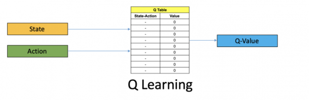
What is Q-Value?
- Q-value (or action-value) is a mapping from state-action pairs to expected future rewards.
- The Q-value is denoted as
Q(s, a).
$$ Q(s, a) = E[R_t | s_t = s, a_t = a] $$
expected future reward if the agent is in state `s` and takes action `a`.Bellman Equation
- The Bellman equation is a recursive equation that relates the value of a state to the values of its successor states.
$$ Q(s, a) = r + \gamma \max_{a’} Q(s’, a’) $$
- Where:
ris the immediate reward received after taking actionain states.γ(gamma) is the discount factor, which determines the importance of future rewards.s'is the next state after taking actionain states.a'is the next action taken in states'.
- The Bellman equation is used to update the Q-value for a given state-action pair.
Temporal Difference Learning
- Temporal difference (TD) learning means, we don’t wait for the final outcome to update the Q-value.
- Instead, we update the Q-value based on the immediate reward and the estimated value of the next state.
It's like:

- You drive 10 meters — it feels good, so you think: "Hey, driving is fun!" (reward!)
- You drive 100 meters and reach KFC — it feels even better!

Now — when you first started, you didn’t know driving 10 meters was leading to the KFC.

Over time, you realize:

- "Ohh, that small 10-meter drive was actually important, because it eventually got me to the KFC!"
Temporal Difference Update Rule
- In Q-learning, we use the TD update rule to update the Q-value for a given state-action pair.
- We’d some initial estimate for the Q-value in some state
sand actiona. When we actually take actionain states, we get a rewardrand move to the next states'with some max Q-value for some possible actiona'. - So, we would like to update the Q-value for the state-action pair
(s, a), but we don’t want to completely forget the previous estimate. Who knows, maybe it was a good estimate. - So, we use a learning rate
α(alpha) to control how much we want to update the Q-value.
$$ Q(s, a) \leftarrow Q_{old}(s,a) + \alpha [Q_{new}(s,a) - Q_{old}(s,a)] $$
$$ Q(s, a) \leftarrow Q(s, a) + \alpha [r + \gamma \max_{a’} Q(s’, a’) - Q(s, a)] $$
Epsilon-Greedy Policy
- Choose the best action with probability
1 - ε(epsilon). - Choose a random action with probability
ε. - This helps the agent to explore new actions and avoid getting stuck in local optima.
Introduce randomness in the action selection process to explore the environment.Q-Learning approach
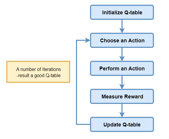
Python Implementation
import numpy as np
import matplotlib.pyplot as plt

# Parameters
n_states = 16
n_actions = 4
goal_state = 15

Q_table = np.zeros((n_states, n_actions))

learning_rate = 0.8
discount_factor = 0.95
exploration_prob = 0.2
epochs = 1000

# Q-learning process
for epoch in range(epochs):
    current_state = np.random.randint(0, n_states)

    while current_state != goal_state:

        # Exploration vs. Exploitation (ϵ-greedy policy)
        if np.random.rand() < exploration_prob:
            action = np.random.randint(0, n_actions)
        else:
            action = np.argmax(Q_table[current_state])

        # Transition to the next state (circular movement for simplicity)
        next_state = (current_state + 1) % n_states

        # Reward function (1 if goal_state reached, 0 otherwise)
        reward = 1 if next_state == goal_state else 0

        # Q-value update rule (TD update)
        Q_table[current_state, action] += learning_rate * \
            (reward + discount_factor * np.max(Q_table[next_state]) - Q_table[current_state, action])

        current_state = next_state  # Update current state

# Visualization of the Q-table in a grid format
q_values_grid = np.max(Q_table, axis=1).reshape((4, 4))

# Plot the grid of Q-values
plt.figure(figsize=(6, 6))
plt.imshow(q_values_grid, cmap='coolwarm', interpolation='nearest')
plt.colorbar(label='Q-value')
plt.title('Learned Q-values for each state')
plt.xticks(np.arange(4), ['0', '1', '2', '3'])
plt.yticks(np.arange(4), ['0', '1', '2', '3'])
plt.gca().invert_yaxis()  # To match grid layout
plt.grid(True)

# Annotating the Q-values on the grid
for i in range(4):
    for j in range(4):
        plt.text(j, i, f'{q_values_grid[i, j]:.2f}', ha='center', va='center', color='black')

plt.show()

# Print learned Q-table
print("Learned Q-table:")
print(Q_table)
Last updated on